Tutorial 3 - Using Python API
- Build Instruction
- Tutorial 1 - Hello, Jet!
- Tutorial 2 - Using Mesh and Surface Set
- Tutorial 3 - Using Python API
- Manual (Feature) Tests
- Unit Tests
- Performance Tests
- Supported Platforms
- C++ API Reference
- Python API Reference
Introduction
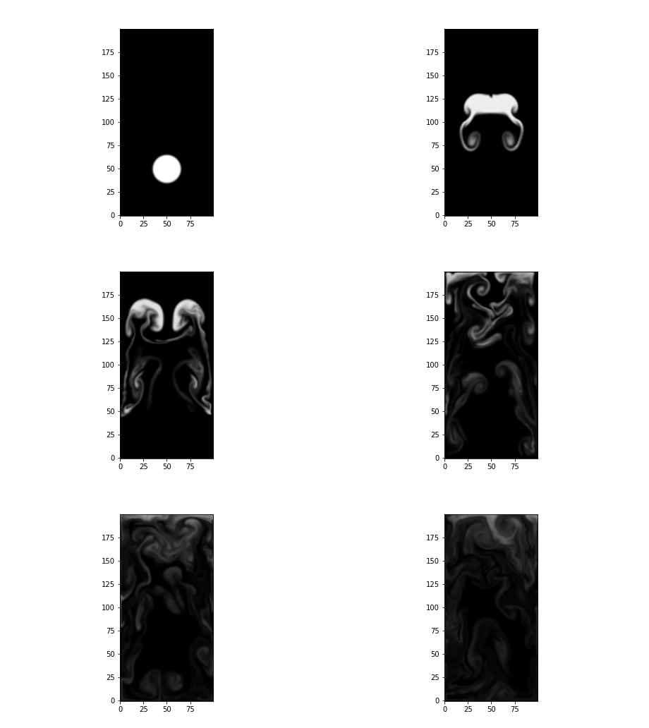
Jet framework also comes with Python API which covers most of the high-level C++ API. In this tutorial, we will see how to use the Python API to create a smoke simulation. Once completed, the result will look like this:

Initial Setup
After installing the framework using pip (see Build Instruction), we can import the module by simply writing:
import pyjet
For the demo purpose, we will just import everything by from pyjet import *. We also want to import a couple of more modules to visualize the simulation, so our skeleton code with full import block is going to be:
from pyjet import *
import sys
import numpy as np
import matplotlib.pyplot as plt
import matplotlib.animation as animation

def main():
    # More codes here

if __name__ == '__main__':
    Logging.mute()
    main()
Note that for the sake of the demo, we are muting the logger.
Writing Simulation
Creating a simulation is very similar to the code using C++ API. For example, to build a 2-D smoke simulator,
...

def main():
    # Create smoke solver
    resX = 100
    solver = GridSmokeSolver2(resolution=(resX, 2 * resX), domainSizeX=1.0)

...
This will build a solver with 100 x 200 resolution grid with 1m x 2m domain.
In this particular example, we want to make the simulation to run at interactive frame rate. In most cases, the linear system solver for the pressure calculation is the bottleneck of the performance. So, let’s try to swap the solver with less accurate, but much faster solver.
...

def main():
    # Create smoke solver
    ...

    # Customize pressure solver
    pressureSolver = GridFractionalSinglePhasePressureSolver2()
    pressureSolver.linearSystemSolver = FdmGaussSeidelSolver2(20, 20, 0.001)
    solver.pressureSolver = pressureSolver

...
We are using GridFractionalSinglePhasePressureSolver2 for the pressure solver which is the same as the default setting. We are only customizing the linearSystemSolver by using FdmGaussSeidelSolver2 instead of FdmIccgSolver2 which is the default configuration.
To create an emitter, we follow nearly the same routine as we did from the C++ world which is:
...

def main():
    # Create smoke solver
    ...

    # Customize pressure solver
    ...

    # Setup emitter
    sphere = Sphere2(center=(0.5, 0.5), radius=0.15)
    emitter = VolumeGridEmitter2(sourceRegion=sphere)
    solver.emitter = emitter
    emitter.addStepFunctionTarget(solver.smokeDensity, 0.0, 1.0)
    emitter.addStepFunctionTarget(solver.temperature, 0.0, 1.0)

...
From the code above, we are creating a spherical volume emitter at (0.5m, 0.5m) with the radius of 0.15m. We then connect that emitter to smoke density and temperature.
Running Simulation
Once the simulation is set up, we can run the sim by simply looping over the frames such as:
...

ANIM_NUM_FRAMES = 360
ANIM_FPS = 60

def main():
    # Create smoke solver
    ...

    # Customize pressure solver
    ...

    # Setup emitter
    ...

    # Run the sim
    frame = Frame(0, 1.0 / ANIM_FPS)
    while frame.index < ANIM_NUM_FRAMES:
        solver.update(frame)
        frame.advance()
...
Quite simple, isn’t it? But without any visualization, it seems a bit boring. So let’s modify the code as shown below:
...

def main():
    # Create smoke solver
    ...

    # Customize pressure solver
    ...

    # Setup emitter
    ...

    # Animation
    frame = Frame(0, 1.0 / ANIM_FPS)
    def updatefig(*args):
        solver.update(frame)
        frame.advance()
        den = np.array(solver.smokeDensity.dataAccessor(), copy=False)
        im.set_data(den)
        return im,

    # Visualization
    fig = plt.figure()
    den = np.array(solver.smokeDensity.dataAccessor(), copy=False)
    im = plt.imshow(den, vmin=0, vmax=1, cmap=plt.cm.gray,
                    interpolation='bicubic', animated=True, origin='lower')
    anim = animation.FuncAnimation(fig, updatefig, frames=ANIM_NUM_FRAMES,
                                       interval=1, blit=True)
    plt.show()
...
For the most of the parts, matplotlib doing its magic. But please take a look at the line:
den = np.array(solver.smokeDensity.dataAccessor(), copy=False)
This line shows how to convert internal data from Jet to NumPy.
Putting All Together
Below is the code that puts everything together into a single program.
from pyjet import *
import sys
import numpy as np
import matplotlib.pyplot as plt
import matplotlib.animation as animation

ANIM_NUM_FRAMES = 360
ANIM_FPS = 60


def main():
    # Create smoke solver
    resX = 100
    solver = GridSmokeSolver2(resolution=(resX, 2 * resX), domainSizeX=1.0)

    # Customize pressure solver for real-time sim (less accurate, but much faster)
    pressureSolver = GridFractionalSinglePhasePressureSolver2()
    pressureSolver.linearSystemSolver = FdmGaussSeidelSolver2(20, 20, 0.001)
    solver.pressureSolver = pressureSolver

    # Setup emitter
    sphere = Sphere2(center=(0.5, 0.5), radius=0.15)
    emitter = VolumeGridEmitter2(sourceRegion=sphere)
    solver.emitter = emitter
    emitter.addStepFunctionTarget(solver.smokeDensity, 0.0, 1.0)
    emitter.addStepFunctionTarget(solver.temperature, 0.0, 1.0)

    # Visualization
    fig = plt.figure()
    den = np.array(solver.smokeDensity.dataAccessor(), copy=False)
    im = plt.imshow(den, vmin=0, vmax=1, cmap=plt.cm.gray,
                    interpolation='bicubic', animated=True, origin='lower')

    # Animation
    frame = Frame(0, 1.0 / ANIM_FPS)
    def updatefig(*args):
        solver.update(frame)
        frame.advance()
        den = np.array(solver.smokeDensity.dataAccessor(), copy=False)
        im.set_data(den)
        return im,

    if len(sys.argv) > 1:
        format = sys.argv[1]
        if format == 'gif':
            anim = animation.FuncAnimation(fig, updatefig,
                                           frames=ANIM_NUM_FRAMES,
                                           interval=ANIM_FPS, blit=True)
            anim.save('smoke_example01.gif', fps=ANIM_FPS, dpi=72,
                      writer='imagemagick')
        elif format == 'mp4':
            anim = animation.FuncAnimation(fig, updatefig,
                                           frames=ANIM_NUM_FRAMES,
                                           interval=ANIM_FPS, blit=True)
            anim.save('smoke_example01.mp4', fps=ANIM_FPS, writer='ffmpeg')
    else:
        anim = animation.FuncAnimation(fig, updatefig, frames=ANIM_NUM_FRAMES,
                                       interval=1, blit=True)
        plt.show()


if __name__ == '__main__':
    Logging.mute()
    main()
For the complete API reference, please visit Python API Reference.